Loading SWATfarmR
You can install SWATfarmR from its GitHub repository. If
you did not install the R package yet, install it with
remotes::install_github().
# If the package remotes is not installed run first:
install.packages('remotes')

remotes::install_github('chrisschuerz/SWATfarmR')
Before we start exploring the package load
SWATfarmR.
Demo data
To work with SWATfarmR we need a SWAT model setup for
which we want to schedule farm management operations and a file in which
we define the management operation sequences and the rules on which we
base the operation scheduling. I will from now on refer to this file as
the management input file. SWATdata provides a set of fast
running, lightweight SWAT2012 and SWAT+ model setups of a head watershed
of the Little River Experimental Watershed (LREW; Bosch et al. (2007)). SWATfarmR comes
with a demo management input file which provides the operation templates
for the SWAT+ model setup that is available from
SWATdata.
Although the code below can also install SWATdata for
you, I recommend to install it before you start working with the example
below. To install SWATdata you can use again the
remotes package.
remotes::install_github('chrisschuerz/SWATdata')Loading the demo data
Demo data can be loaded with the function load_demo().
With the input argument dataset you define which data you
want to load. To load a SWAT project simply define
dataset = 'project'. The path defines the path
on your local hard drive where you want to store the SWAT project
folder. Please try to avoid blanks in your path
names (e.g. ‘C:/this is a/path with blanks’).
This can cause issues when running the model. Try to use
e.g. ’_’ in your path names
instead. As the SWAT project is available as SWAT+ and as
SWAT2012 project you have to specify the version of the
SWAT project you want to load. At the moment there is only a demo for
SWAT+ available. So, use version = 'plus' to load a SWAT+
project
.
# The path where the SWAT demo project will be written
demo_path <- 'Define:/your/path'

# Loading a SWAT+ demo project
proj_path <- load_demo(dataset = 'project',
                       path = demo_path,
                       version = 'plus')
When you load a SWAT project load_demo() saves the
defined SWAT project in the file path that was defined with
path = demo_path and returns the final demo project path as
a character string in R. I assigned the output of
load_demo to the variable proj_path to use
this path later with SWATfarmR.
If you set dataset = 'schedule' you can load the demo
management input file for the SWAT+ demo project. Again use
path = demo_path to define the path where the csv
file is written. Although there is only a demo management input file
available for SWAT+ available at the moment you have to define
version = 'plus'.
# Loading a SWAT+ demo project
mgt_path <- load_demo(dataset = 'schedule',
                      path = demo_path,
                      version = 'plus')
#> Warning in load_demo(dataset = "project", path = demo_path, version = "+"): Demo
#> already exists in provided 'path'. To work with the existing demo project use
#> the returned path.Again load_demo() returns the path of the csv
file as a character string in R which will be useful in our
SWATfarmR workflow. I assigned the file path to the
variable mgt_path. The management input file is key to
control the management scheduling with SWATfarmR. Setting
up this file requires to keep a very clear file structure. For the rules
which control the management scheduling you can make use of several
variables which eventually affect the operation dates that will be set
in the management schedules. So it is worth to have a detailed look into
this file.
The management input file
The SWATfarmR workflow reads the management operations
from a csv file. Depending how complex you define the
management to be for a SWAT model setup this file can be rather long.
The csv file can be edited and prepared in any spreadsheet
software, such as Excel or Libre office Calc which may be easier than
processing the file in R.
The image below shows a minimum example for a management input file
for a SWAT+ model setup. The columns land_use,
management, weight,
filter_attribute, and
condition_schedule are the same for SWAT2012 and SWAT+
and are required in the table even if they are left empty. The remaining
columns are SWAT version dependent and are the actual operation
parameters which are written into the management schedules of the SWAT
model input files. SWAT+ management operations consist of the
operation type and three parameters for each operation
which are called op_data1, op_data2,
and op_data3. These names are used as column names in
the management input file. SWAT2012 management inputs also use different
operation types, but each operation can be controlled
by 9 different parameters mgt1 to
mgt9. Thus the SWATfarmR management input
must be prepared for SWAT2012 model setups accordingly. The following
explanations only address the use of SWATfarmR with SWAT+
model setups. An application with SWAT2012 may be added in the
future.
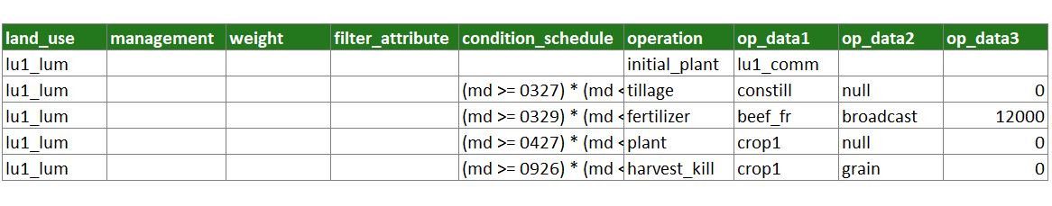
Fig. 1: Minimum example of a management input file. The table shows only operations for one land_use and one crop. In the example no management alternatives and filter_attributes would be applied.
In the land_use column all operations that belong to one land use are grouped together. In the small example above all 5 operations should be scheduled for the land use ‘lu1_lum’. All land uses which are defined in land_use must be defined in the file ‘landuse.lum’ and must be assigned to HRUs in ‘hru-data.hru’. Otherwise this management will not be implemented in the model setup.
The columns management and weight are always used together. These provide the option to randomly distribute different managements in a model setup. A SWAT modeler can have for example statistical data on the implementation of conservation farming, but no data is available on the actual locations of implementation. Then management and weight allow a random distribution of e.g. different tillage types in the catchment based on weighted random sampling using the provided weights. Providing information in these columns is optional. Thus in most cases management and weight are left empty.
With filter_unit the user has the option to apply operations only to HRUs which fulfill certain criteria which are defined here. These criteria can for example be a slope threshold, soil type or location (in defined routing units). Below this will be further explained. Providing such criteria is optional and in most cases filter_unit is left empty.
The most important column is condition_schedule in which you define the temporal conditions for scheduling an operation. The conditions which can be defined here are very flexible and endless combinations are possible to control the operation scheduling. This flexibility is however also a potential source for error. Thus the definition of scheduling conditions will be covered in great detail below.
operation and the corresponding parameters op_data 1 to 3 define the actual SWAT management. All management operations and parameters which are defined here must be defined in the SWAT model setup to work. If for example a fertilizer application is defined then op_data1 defines the fertilizer type. In the example above ‘elem_n’ is applied. This fertilizer type must then be defined in the SWAT+ input file ‘fertilizer.frt’.

Fig. 2: Schematic workflow of filtering operation schedules based on land_use, management, and filter_attribute
land_use
The land_use label defines to which land use class
the sequences of operations that are defined in the table belong to.
When the scheduling routine of SWATfarmR iterates over all
HRUs, the routine filters all operations from the management input table
where the land uses in the column land_use match the
HRUs land use (which is defined in the file ‘hru-data.hru’. See
the figure above.). This means that you must be careful how you define
the land uses in the management input table. Not match land use labels
are ignored in the scheduling (e.g. in the case of typos). If you
accidentally put an operation sequence for a land use into the table
twice all these data will be used in the operation scheduling (so be
careful when copy/pasting!).
management and weight
With management and weight you can introduce different management types that you want to apply to HRUs with weighted random sampling. This is useful when you want to translate statistical information into the farm management in a SWAT model setup.
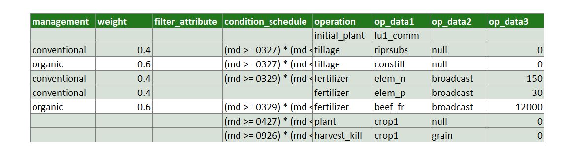
Fig. 3: Filtering operations based on different management alternatives.
Let us assume that in the example above we know from agricultural statistics that for the land_use ‘lu1_lum’ (which was selected for the current HRU) 40% of the farmers do conventional farming and 60% do organic farming. For the different practices we want to implement different tillage types and fertilizer types and amounts. In the management input file we introduce two different managements for all tillage and fertilizer operations. You can select any names for the two different managements. You just have to be consistent with the names for all operations that you want to introduce as alternatives. The percentages of the two farm practices we add as weights for the respective operations. The tillage alternatives only differ in the selected plough type. For the fertilizer operations you can see that ‘conventional’ uses two fertilizer operations while ‘organic’ does one manure application. For all other operations that should be used in both managements just keep the management and the weight columns empty. In the example table you can see that the ‘conventional’ alternative was selected for the current HRU. The white rows in the table will be removed from the operation scheduling of this HRU.
filter_attribute
There are cases where we want to use the same management practice
sequences (e.g. the same crop rotation) for different HRUs, but we want
to introduce some different operations because of some any HRU
attributes. You might want to use different tillage practices for
different soils, or want to apply contour farming on steeper slopes, or
you for example know that the amounts of fertilizer differ between
regions (which may correspond to routing units or subbasins in your
model setup). Similar to the different managements above you can also
select the operation that should be scheduled for an HRU, based on the
HRUs attributes. Below you can see the hru_attributes table
of a SWATfarmR project. It shows all attributes that
implemented to select operations at the moment.
#> # A tibble: 49 × 9
#>      rtu rtu_name   hru hru_name lu_mgt    soil      slp slp_len hyd_grp
#>    <dbl> <chr>    <dbl> <chr>    <chr>     <chr>   <dbl>   <dbl> <chr>
#>  1     1 rtu10        1 hru01    agrl4_lum LREW06 0.0309      60 B
#>  2     1 rtu10        2 hru02    agrl1_lum LREW06 0.0327      60 B
#>  3     1 rtu10        3 hru03    agrl1_lum LREW10 0.0282      90 D
#>  4     1 rtu10        4 hru04    agrl1_lum LREW09 0.0215      90 C
#>  5     1 rtu10        5 hru05    frse_lum  LREW06 0.0432      60 B
#>  6     1 rtu10        6 hru06    frse_lum  LREW03 0.0386      60 B
#>  7     1 rtu10        7 hru07    frse_lum  LREW10 0.0321      60 D
#>  8     1 rtu10        8 hru08    frse_lum  LREW05 0.0460      60 B
#>  9     1 rtu10        9 hru09    frse_lum  LREW08 0.0582      30 C
#> 10     1 rtu10       10 hru10    agrl2_lum LREW03 0.0363      60 B
#> # … with 39 more rows
#> # ℹ Use `print(n = ...)` to see more rows
The attributes that can be useful in practice are rtu,
soil, slp, slp_len, and
hyd_grp. You can use and combine filter conditions for
these attributes in many different ways. You should however clearly
consider the consequences for the operation scheduling when you filter
operations based on HRU attributes. In the schematic workflow in Fig. 2
you can for example see that I introduced 2 conditions which complement
each other. By conditioning one operation with
slp >= 0.08 and a second one with
slp < 0.08 one of the two operations will be used and
there will not be a case where none or both operations are kept in the
operation schedule. Below I show a few small examples for conditions to
filter based on HRU attributes.
If you want to use a specific operation for example only in the management schedules of the routing units 1 to 5, 7, and 10 you could for example use the following condition:
If you add this condition for one operation but you do not provide an alternative all other routing units will not use an alternative to this operation. To provide an alternative for all other locations you can for example use the following condition for the alternative operation:
To apply an operation only for the soil ‘LREW06’ you can use the following:
soil == 'LREW06'The alternative again would be:
soil != 'LREW06'If you want to consider several soils, this is the way to do it:
You can also combine conditions:
This operation would be implemented for all HRUs with a soil type that is not ‘LREW06’ for the routing units 1 to 5, 7, and 10 and only on slopes lower equal to 0.08.
condition_schedule
condition_schedule controls the temporal scheduling
of the management operations. The condition definition works in similar
to the attribute filtering with filter_attribute. The
main difference is that filter_attribute requires
either TRUE or FALSE as a result from the
filter condition to decide whether an operation is scheduled for an HRU
or not. condition_schedule, however, allows to assign
probabilities to dates based on the defined conditions to control “how
likely” it is that an operation takes place on a certain day. Similar to
filter_attribute there are a few default variables that
the user can use to define scheduling conditions. The table below
summarizes them.
| Variable | Definition | Usage |
|---|---|---|
prev_op |
Date of the previous operation in <date>
format. |
2000-01-01 |
date |
Date of the actual operation in <date>
format. |
2000-01-01 |
year |
Year of a date in a 4 digit integer format. | 2000 |
month |
Month of a date as integer value. | Numbers 1 to 12 |
day |
Day of a date as integer value. | Numbers 1 to 31 |
jdn |
Julian of a date as integer value. | Numbers 1 to 366 |
md |
Month and day of a date as a combined integer value. | e.g. 101 (Jan. 1), 1125 (Nov. 25) |
ymd |
Month and day and year of a date as a combined integer value. | e.g. 20000101 (Jan. 1 2000) |
pcp |
Daily precipitation sum for a certain date in mm. | 1.23 |
tmax |
Maximum daily temperature for a certain date in mm. | 1.23 |
tmin |
Minimum daily temperature for a certain date in mm. | 1.23 |
tav |
Average daily temperature for a certain date in mm. | 1.23 |
hu_<crop> |
SWAT+ specific. Heat units of a crop at a certain date
after planting and before harvesting that crop. Replace |
hu_wwht for winter wheat |
grw_<crop> |
SWAT+ specific. Days a crop is already growing after
planting that crop. Replace |
grw_wwht for winter wheat |
hu |
SWAT2012 specific. Heat units of a crop at a certain date
after planting and before harvesting that crop. No |
|
hu_fr |
SWAT2012 specific. Heat unit fraction of a crop at a
certain date after planting and before harvesting that crop. No hu and the heat units that
were defined for a crop when planting. |
Fig. 4 again shows the management input from the previous examples after selecting all rows where land_use is ‘lu1_lum’ and after selecting the ‘conventional’ management and filtering the operations by specific HRU attributes. You can immediately see two things in the column condition_schedule. The conditions do have a similar structure as the conditions for filter_attribute and that there are operations where condition_schedule is left empty.
An empty condition_schedule can have two functions:
- The operation
initial_plantdoes not use any conditions to set the operation.skipcan be triggered with conditions but does not necessarily need one. - For other operations (e.g.
fertilizerapplication ofelem_pin Fig.4) leaving condition_schedule empty results in scheduling this operation at the same date as the previous operation.
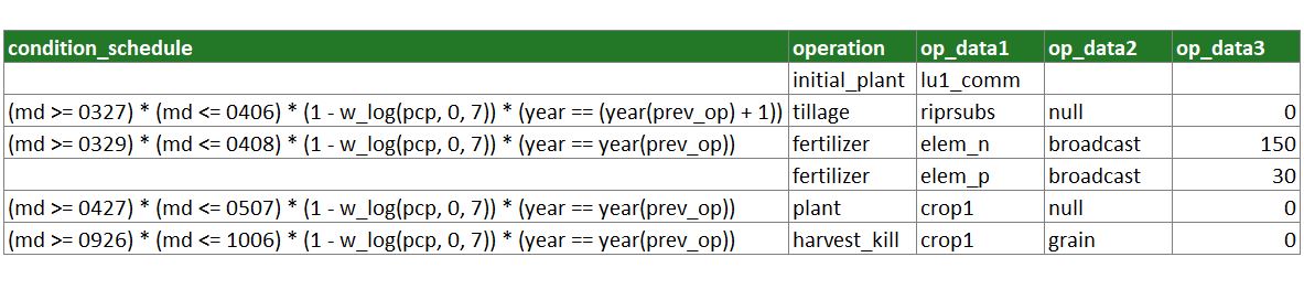
Fig. 4: Example for operation schedule with temporal conditions.
All conditions that were implemented to control the scheduling of the
operations in the example in Fig. 4 follow almost the same pattern. The
condition for the plant operation for example is the
following:
(md >= 0427) * (md <= 0507) * (1 - w_log(pcp, 0, 7)) * (year == year(prev_op))You can see that it uses the variables md,
pcp, year, and prev_op that are
listed in the table above. Further the condition uses the two functions
w_log() and year(). year() is
available from the R package lubridate and
returns the year of a date as an integer value. w_log() on
the other hand is a function that was included in
SWATfarmR. The function implements a logistic function to
calculate weights with a smooth transition between an upper and lower
value. Besides w_log() there is also w_lin()
which does a linear transition between the upper and the lower value.
Below you can see how the two functions look like. A major difference
between the two functions is that w_log() converges to 0
and 1 at its boundaries, but does not reach these values, while
w_lin() reaches 0 and 1 at its boundaries. Overall I always
prefer to use w_log() in the condition definition as it is
safer to not risk of having all probabilities for an operation 0 but
very low and thus risking to skip the scheduling of an operation. This
can however happen more easily with w_lin() resulting in
0.
x <- seq(-0.5,1.5, length.out = 100)
log_wgt <- w_log(x, 0, 1)
lin_wgt <- w_lin(x, 0, 1)

plot(x, log_wgt, type = 'l', col = 2, ylab = 'weight')
lines(x, lin_wgt, col = 4, lty = 2)

legend("topleft", legend=c("w_log", "w_lin"),
       col=c("red", "blue"), lty = 1:2, cex=0.8)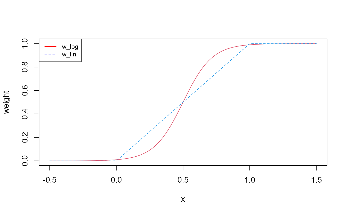
Fig. 5: Functional relationship of a variable with the two weight functions w_log() and w_lin().
We will now go through the individual conditions that were combined
by multiplying them. The first two conditions use md. In
the first expression md >= 0427, which means the
combination of month and day must be larger or equal to 427. This
translates to a date in any year later or equal than April 27. The
second expression translates to all dates in any year earlier or equal
to May 7. When we multiply those two expressions all dates between April
27 and May 7 get a probability of 1 while all dates outside of this time
window do have a probability of 0.
(md >= 0427) * (md <= 0507)The third expression uses the w_log() function together
with precipitation. The second and third input argument in the function
define the lower and upper boundary values of the transition range. In
this case w_log() returns the value 0.01 when
pcp = 0 and a value 0.99 when pcp = 7.
(1 - w_log(pcp, 0, 7))Plotting the function shows the intention of this condition. We assign to all daily precipitation values of 0 mm a weight of (almost) 1. Yet, precipitation sums of 2 mm still result in a probability of 0.88 while at 4 mm the probability dercreases to 0.34. Daily precipitation sums of larger than 7 mm receive a weight of (almost) 0. This condition makes the scheduling of operations on days that exceed a certain precipitation less likely.

Fig. 6: Example for using w_log() to assign lower weights to days with higher precipitation.
We can now combine all 3 conditions and use this combination for
scheduling the plant operation. When we compare the time
series of precipitation and the weights based on precipitation we can
see that all days without precipitation get a weight of 1 while rainy
days will have a weight lower than one. The red bars show the combined
weights for all days. You can see that the conditions with
md define the time window between April 27 and May 7. In
this time window dates are then excluded or have a lower weight
depending on the precipitation on these dates. The operation scheduling
algorithm selects a date for an operation with weighted random sampling.
Thus all dates with a weight > 0 can be selected. Dates with larger
weights are however more likely to be selected than dates with smaller
weights.
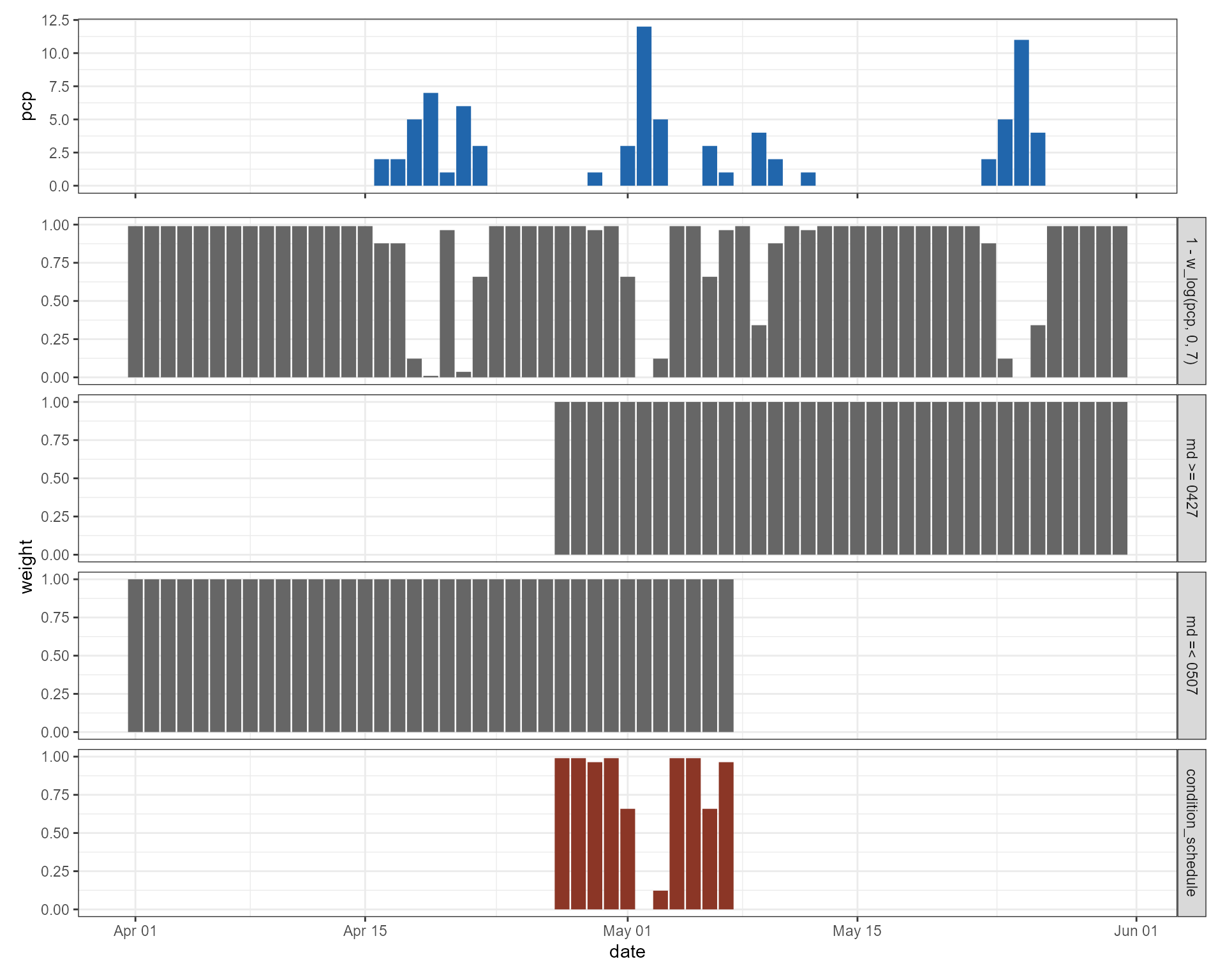
Fig. 5: Combination of 3 conditions to a combined condition for scheduling an operation.
The fourth element of the entire scheduling condition refers to the
year. This is necessary because the md conditions only
constrain the time window by month and day. This time window is however
given in the current year of scheduling, but also in all future years.
Thus, there is a risk that the scheduling of an operation skips years.
To avoid the skipping of years I strongly recommend to add a constrain
that the current operation must be scheduled in the same year as the
previous operation.
(year == year(prev_op))This constrain does however not apply to the first operation or the first operation of any year in a crop rotation. In this case you can, however, define that this operation should take place in the year that is the year of the previous operation plus 1.
(year == year(prev_op) + 1)operation and op_data
The columns operation, op_data1, op_data2, and op_data3 are eventually written into the ’management.sch’ input file of the SWAT+ model setup. Different operations require different op_data parameters. Please refer to the SWAT+ documentation to learn how to define the parameters for the management operations.
A selection of operations are available in SWAT
which you can trigger in a SWAT simulation. The table below lists the
SWATfarmR labels and their corresponding SWAT+ labels.
SWATfarmR code |
SWAT+ code | Definition |
|---|---|---|
| plant | plnt | Planting operation |
| irrigation | irrm | Irrigation operation |
| fertilizer | fert | Fertilizer application |
| pesticide | pest | Pesticide application |
| harvest_kill | hvkl | Harvest and kill the plant |
| tillage | till | Tillage operation |
| harvest_only | harv | Only harvest the plant (or a part of the plant) |
| kill_only | kill | Kill the plant |
| grazing | graz | Grazing operation |
| street_sweeping | swep | Sweeping operation |
| burn | burn | Burning operation |
| skip | skip | Skip a year |
| initial_plant | inip | Define the initial crop |
The only non-SWAT specific operation in the table above is
initial_plant. This is a required input for every
land_use that is defined in the management input file.
The initial_plant must refer to a plant community that is
defined in the ‘plant.ini’ SWAT+ input file.
A new SWATfarmR project in R
SWATfarmR uses an object based approach to work with
your SWAT project. This means that when you start a new
SWATfarmR project an object (I will call it
farmr project or farmr object, if I refer to
the R object, from now on) will be generated in your
R environment. The farmr project stores
relevant data of your SWAT project, such as the weather data or HRU
attributes and provides functions to work with theses data and
eventually allows you to schedule management operation for your SWAT
project. In this small example we will use the demo data that I
described in the section Demo
data above. If you did not load the demo project and the demo
management input file yet, please do that before you continue. To start
a new farmr project use the function
new_farmr(). The function requires two inputs. First you
have to name your project. This will be the name of your
farmr project in R and the name of the
‘.farm’ file in your SWAT project folder. If you want to
generate several farmr projects for a SWAT project, they
have to have different names. The function also requires the path of
your SWAT project on the hard drive as an input argument. In this
example I will call the farmr project
lrew_demo and will use the path of the demo SWAT project
proj_path which we already defined in the section Demo
data.
new_farmr(project_name ='lrew_demo',
          project_path = proj_path)

#>  Finished in 1S
Now have a look in to your R variables. There is now a
new object called lrew_demo which is our farmr
project. You will also find the file ‘lrew_demo.farm’ in your
SWAT project folder. This is the file where all your work with in your
farmr project will be saved and from which you can load
your farmr project to continue with your work.
A quick look into the farmr object
You can now start exploring the generated farmr object
in R. To see all elements that are in the new project you
can use the $ operator, like you would access elements of a
list in R. Fig. 6 shows a screenshot of the new
farmr object and the suggestions to select an element after
entering the $ operator. The first 4 elements are functions
to apply operations to your farmr project. The last element
.$.data holds the data that was read from the SWAT project,
such as the weather inputs ‘pcp’ and ‘tmp’ or HRU
attributes.
From the 4 functions, only .$add_variable() and
.$read_management() are relevant to you as a user.
.$initialize() is synonymous to new_farmr()
which we already performed. With .$save() you can save the
current state of the farmr project at any time. Saving is
however done after each operation automatically. Thus, manually saving
should not be necessary. After executing some of the functions and
working through the operation scheduling, new functions will be
activated (e.g. after reading the management input with
.$read_management() the function
.$schedule_operations() becomes visible).
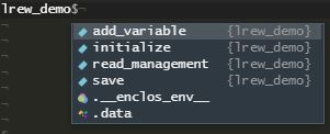
Fig. 6: Screenshot of the new farmr
object in R.
Reading the management input
We will now read the management input file for the demo project which
we saved on the hard drive in the path mgt_path into the
farmr project. This is done with the function
.$read_management().
lrew_demo$read_management(file = mgt_path)

#> Warning: No management schedules were found for the following SWAT land uses:
#>   utrn_lum, urml_lum
#>   If managements should be written for any of these land uses
#>   please add them to the management table and read the table again.
You can see that loading the management input file triggers a warning
message. The management input file does not define any management for
the land uses ‘utrn_lum’ and ‘urml_lum’. In this case
this is OK and we can ignore the warning message as we do not want to
apply any management to the urban land uses. If the warning message
however lists land uses of your model setup for which you intend to
implement a management you should go back to your management input file,
include the managements for the missing land uses and load it again with
.$read_management(). Besides the input argument
file, .$read_management() also has a second
input argument discard_schedule. You can ignore this when
reading a management into a new farmr project. You have to
set this however discard_schedule = TRUE if you already
scheduled operations with an other management input file, but you want
to change the management inputs. Then the already scheduled operations
would not match the new management input file that you plan to read. In
this case you would have to discard the already scheduled
operations.
Reading the management input into our farmr project
lrew_demo unlock the function
.$schedule_operations(). With
.$schedule_operations() we can schedule management
operations based on the operations and conditions that we defined in the
management input file. We can just try to run the operation scheduling
and see what happens.
lrew_demo$schedule_operations()

#> Scheduling operations:
#> Error in `mutate()`:
#> ! Problem while computing `wgt = ... * (year == (year(prev_op) + 1))`.
#> Caused by error in `w_log()`:
#> ! object 'api' not found
#> Backtrace:
#>   1. lrew_demo$schedule_operations()
#>  10. SWATfarmR::w_log(api, 5, 20)
Scheduling operations triggered an error. A closer look into the
error message tells us that object 'api' not found and that
the error occurred in SWATfarmR::w_log(api, 5, 20). This
looks like one of the operation conditions in the management input file.
If you have a look into the demo management input file you can see that
I actually included the variable api into the scheduling
conditions with the function (1 - w_log(api, 5, 20)). The
variable api is however no default variable (see again the
table in the subsection condition_schedule)
and we have to add this variable to the farmr project if we
want to use it in the scheduling conditions.
Adding variables
My intention with the api condition was to include the
antecedent precipitation (api = antecedent precipitation index) as a
condition for the operation scheduling. A disadvantage of
SWATfarmR compared to decision tables in SWAT+ is that the
operation scheduling with SWATfarmR cannot make use of the
values of any state variables during the simulation which is possible
with decision tables. While for example decision tables can use the soil
moisture as a condition, SWATfarmR must use a proxy
variable which is related to the “wetness” of the soil.
Excursus variable_decay()
One approach to account for the precipitation of previous days would
be to calculate the precipitation sums for a certain number of days
before the current day. This might however not be the best approach to
do that. As an alternative approach, I included a function called
variable_decay() in SWATfarmR which assigns
weights to previous days based on exponential decay. The example below
shows how the weight of an event on day 1 changes for following days.
Depending on the decay_rate the weight of day 1 would only
have a weight of 0.37 for a decay_rate = 1, but still be
accounted with 0.78 with a decay_rate = 0.25. The event on
day 1 would not have much impact from day 5 on for
decay_rate = 1, but would still have a weight of 0.37 for
decay_rate = 0.25.
x <- data.frame(x_1 = c(1,0,0,0,0,0,0,0,0,0,0))
y1<- variable_decay(variable = x, n_steps = -10, decay_rate = 1)
y2<- variable_decay(variable = x, n_steps = -10, decay_rate = 0.8)
y3<- variable_decay(variable = x, n_steps = -10, decay_rate = 0.25)

plot(y1$x_1, type = "l", col = 1, ylab = 'weight', xlab = 'day')
lines(y2$x_1, col = 2)
lines(y3$x_1, col = 3)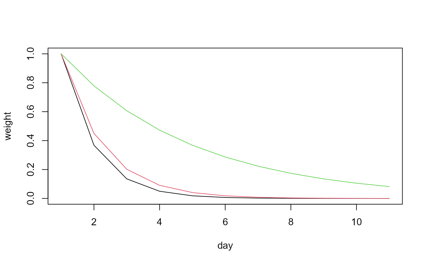
Fig. 7: The effect of decay_rate on the
variable_decay() function.
The small example below should illustrate how we can use
variable_decay() to account for antecedent precipitation.
The black bars in the plot are daily precipitation sums. I calculated
variable_decay() including the 5 previous days
(time_steps <- -5) and used the two rates 0.25 (black
line) and 1 (red line). If we would condition api now with
the rule that triggered the error above
((1 - w_log(api, 5, 20))) we would get lower probabilities
for the days after the large precipitation event on day 4 for both api
time series. While the red line would be already below 5 mm on day 6,
the black line does not fall below 11.5 mm. Thus, in the case of the
black line several days after a rain event would have lower weights in
the operation scheduling. The behaviors of the two api lines could
e.g. be translated to different water retention behaviors of different
soils.
pcp <- data.frame(pcp_1 = c(0,3,7,15,2,0,0,5,2,0))

time_steps <- -5

rate1 <- 0.25
api1 <- variable_decay(pcp, time_steps, rate1)

rate2 <- 1
api2 <- variable_decay(pcp, time_steps, rate2)

plot(pcp$pcp_1, ylim = c(0,22), type = 'h',
     ylab = 'pcp, api', xlab = 'day')
lines(api1$pcp_1, col = 1)
lines(api2$pcp_1, col = 2)
Fig. 8: Two different api time series based on precipitation input and different decay rates
Including api into lrew_demo
We now want to include a new variable api into the
SWATfarmR project lrew_demo which uses the
function variable_decay() to account for the antecedent
precipitation. api in each HRU will be based on the
precipitation time series that is linked with an HRU. In this small
example we also want to account for different hydrological soil groups
(HSG) to consider faster (hsg == 'A') and slower
(hsg == 'D') soil water retention. Be aware that the
approach below works in such a simple way as we only have one weather
station for the entire demo watershed. In a more complex example with
several weather stations you also must account for the links between
weather stations and HRUs. Thus, this would also require to calculate
all combinations of weather stations and HSGs, which would result in
more than only 4 api variables. In a first step we will
extract the precipitation data and the HSG information for all HRUs from
lrew_demo$.data.
# Load dplyr. We will use functions such as 'mutate' and 'select'.
library(dplyr)
# Extract the precipitation from the farmr project
pcp <- lrew_demo$.data$variables$pcp

# Extract the hydrologic soil group values for all HRUs
hsg <- select(lrew_demo$.data$meta$hru_attributes, hru, hyd_grp)
In a next step we calculate different apis based on the
precipitation data pcp, but using different
decay_rates for the different HSGs. The values that I set
here for the decay rates are no literature values and were only chosen
for demonstration of the concept here. In an actual study the choice of
values for decay_rate would need some supporting
literature. We combine the variables api_A to
api_D together into one table and assign the names
'api_A' to 'api_D' to the columns.
# Calculate api values for the hsg classes A to D
api_A <- variable_decay(variable = pcp, n_steps = -5, decay_rate = 1)
api_B <- variable_decay(variable = pcp, n_steps = -5, decay_rate = 0.8)
api_C <- variable_decay(variable = pcp, n_steps = -5, decay_rate = 0.7)
api_D <- variable_decay(variable = pcp, n_steps = -5, decay_rate = 0.5)

# Bind the data together into one api table and name them with the hsgs
api <- bind_cols(api_A, api_B, api_C, api_D)
names(api) <- c('api_A', 'api_B', 'api_C', 'api_D')
This is how the final api table looks like.
api
#> # A tibble: 9,131 × 4
#>     api_A api_B api_C api_D
#>     <dbl> <dbl> <dbl> <dbl>
#>  1 20.3   20.3  20.3  20.3
#>  2 30.3   32.0  33.0  35.2
#>  3 11.2   14.4  16.4  21.3
#>  4  4.11   6.46  8.13 12.9
#>  5  1.51   2.90  4.04  7.85
#>  6  8.18   8.92  9.62 12.4
#>  7  5.50   6.38  7.01  9.04
#>  8  7.05   7.76  8.22  9.42
#>  9  2.59   3.49  4.08  5.72
#> 10  0.954  1.57  2.03  3.47
#> # … with 9,121 more rows
#> # ℹ Use `print(n = ...)` to see more rows
We now generated four different time series for api
depending on different retention behaviors based on the HSGs A to D. For
the implementation in the farmr object we have to link the
different api time series to spatial units of the model
setup. Thus, the table to link variables and spatial units must have two
columns, one for the ids of the spatial units and one for the variable
link. We could link e.g. on a routing unit level if we would use
rtu ids, or to HRUs by assigning an api column
to each hru id in the model setup. In this case we link
HRUs and our new variable. The only variable that determines the link of
the api columns with the HRUs is the HSG of an HRU. We
already extracted hsg above and will now link the
hrus with the apis, by creating a table with
the columns hru and api.
# To add the variable to the farmR you have to tell it which variables are
# assigned to which HRUs
hru_asgn <- mutate(hsg, api = paste0('api_', hyd_grp)) %>%
  select(hru, api)
A quick look at the table shows as how the links between HRUs and
api looks like.
hru_asgn
#> # A tibble: 49 × 2
#>      hru api
#>    <dbl> <chr>
#>  1     1 api_B
#>  2     2 api_B
#>  3     3 api_D
#>  4     4 api_C
#>  5     5 api_B
#>  6     6 api_B
#>  7     7 api_D
#>  8     8 api_B
#>  9     9 api_C
#> 10    10 api_B
#> # … with 39 more rows
#> # ℹ Use `print(n = ...)` to see more rows
We prepared all information that we need to add a new variable. We
can add now the new variable to the farmr object with the
function .$add_variable(). The data we want to
add is the table api that we prepared. The added data must
have the same number of rows as all other variables that are already in
the farmr object. This is ensured in this case as we used
pcp from lrew_demo to calculate
api. We assign the variable name = 'api' to
the new variable in lrew_demo. The name must match the
variable name that is used in the operation conditions of the management
input file and must be different to the names of the already existing
variables. The third input argument assign_unit links the
new variable to the HRUs. Above we defined the links between
hrus and apis in the table
hru_asgn which we will now pass to
.$add_variable.
# Add the variable api to the farmR project
lrew_demo$add_variable(data = api, name = 'api', assign_unit = hru_asgn)
We can now check if the new variable api is available in
lrew_demo. api should be available in
lrew_demo$.data$variables$api.
lrew_demo$.data$variables$api
#> # A tibble: 9,131 × 5
#>    date        api_A api_B api_C api_D
#>    <date>      <dbl> <dbl> <dbl> <dbl>
#>  1 1988-01-02 20.3   20.3  20.3  20.3
#>  2 1988-01-03 30.3   32.0  33.0  35.2
#>  3 1988-01-04 11.2   14.4  16.4  21.3
#>  4 1988-01-05  4.11   6.46  8.13 12.9
#>  5 1988-01-06  1.51   2.90  4.04  7.85
#>  6 1988-01-07  8.18   8.92  9.62 12.4
#>  7 1988-01-08  5.50   6.38  7.01  9.04
#>  8 1988-01-09  7.05   7.76  8.22  9.42
#>  9 1988-01-10  2.59   3.49  4.08  5.72
#> 10 1988-01-11  0.954  1.57  2.03  3.47
#> # … with 9,121 more rows
#> # ℹ Use `print(n = ...)` to see more rows
The connections between variables and HRUs are saved in the table
hru_var_connect. We can see that besides the initially
existing variables pcp, tmax,
tmin, and tav which link to the weather
station, there is now a new column that links to the api
columns that we generated.
lrew_demo$.data$meta$hru_var_connect
#> # A tibble: 49 × 9
#>      rtu rtu_name   hru hru_name pcp    tmax     tmin     tav      api
#>    <dbl> <chr>    <dbl> <chr>    <chr>  <chr>    <chr>    <chr>    <chr>
#>  1     1 rtu10        1 hru01    pcp144 lrew_tmp lrew_tmp lrew_tmp api_B
#>  2     1 rtu10        2 hru02    pcp144 lrew_tmp lrew_tmp lrew_tmp api_B
#>  3     1 rtu10        3 hru03    pcp144 lrew_tmp lrew_tmp lrew_tmp api_D
#>  4     1 rtu10        4 hru04    pcp144 lrew_tmp lrew_tmp lrew_tmp api_C
#>  5     1 rtu10        5 hru05    pcp144 lrew_tmp lrew_tmp lrew_tmp api_B
#>  6     1 rtu10        6 hru06    pcp144 lrew_tmp lrew_tmp lrew_tmp api_B
#>  7     1 rtu10        7 hru07    pcp144 lrew_tmp lrew_tmp lrew_tmp api_D
#>  8     1 rtu10        8 hru08    pcp144 lrew_tmp lrew_tmp lrew_tmp api_B
#>  9     1 rtu10        9 hru09    pcp144 lrew_tmp lrew_tmp lrew_tmp api_C
#> 10     1 rtu10       10 hru10    pcp144 lrew_tmp lrew_tmp lrew_tmp api_B
#> # … with 39 more rows
#> # ℹ Use `print(n = ...)` to see more rows
Scheduling operations
lrew_demo now contains a management input file and all
the required variables that are used in the scheduling conditions. So we
can start scheduling management operations. We can again use the
function .$schedule_operations() that was unlocked after
reading the management input file. .$schedule_operations()
has three input arguments.
The first two input arguments are start_year and
end_year. By default .$schedule_operations()
would schedule farm management operations for the entire time period
that is available from the variable time series. Above you can see that
the date of api starts in 1988 (and ends in
2012). This is the available time period of the weather data that was
used in the model setup process. Scheduling farm management operations
can be quite time intensive and may run several hours for larger model
setups. Thus I recommend to constrain the time window for the operation
scheduling to a shorter time period if any time period outside of the
defined time window would never be used in simulations. Be aware that if
you want to use a time period that is not covered by
start_year and end_year would require to
repeat the scheduling.
The third input argument is n_schedule which is useful
to speed up the scheduling process a bit by reducing the number of
different schedules. n_schedule controls how many different
schedules per land use and routing unit will be generated. Default a
unique operation schedule will be generated for each HRU. If
e.g. n_schedule = 1 a schedule will be generated for a
certain land use in a routing unit and all other land uses within the
same routing unit would use the same schedule. Our small demo watershed
for example only consists of one routing unit with 49 HRUs. 3 HRUs use
the land use ‘lrew_ag1’. In this case only 1 schedule would be
generated if n_schedule = 1 and the other two HRUs would
use the same schedule (which saves computation time as the scheduling
process would simply be skipped for those 2 HRUs). If e.g
n_schedule = 2 the first 2 HRUs would get different
schedules and the third HRU would select one of the two existing
schedules randomly.
In our simple example we want to generate operation schedules for the time window 2000 to 2008. We will only generate two individual schedules per land use.
lrew_demo$schedule_operations(start_year = 2000, end_year = 2008, n_schedule = 2)

#> Scheduling operations:
#>  HRU 1 of 49   Time elapsed: 0S   Time remaining: 48S
#>
#> Scheduling operations:
#>  Finished scheduling 49 HRUs in 11S
Writing operations
When the scheduling was successful we can write the scheduled
operations into the SWAT project using the function
.$write_operations(). .$write_operations()
again uses the two optional input arguments start_year and
end_year. Within the scheduled time window we can select a
shorter time window to write the operations for. This is for example an
interesting option if you want to only write the operations for the
calibration time period, run the simulations to calibrate the model and
then rewrite the management for the validation period. If
start_year and end_year are not used the
entire time period that was scheduled will be written into the
management files. For the demo project we will write the management in
the time window 2000 to 2005.
lrew_demo$write_operations(start_year = 2000, end_year = 2005)

#> Writing management files:
#>   - Writing 'hru-data.hru'
#>   - Writing 'landuse.lum' and 'schedule.mgt'
#>   - Writing 'time.sim'
#> Finished writing management schedules in 1S
From the output message you can see that for a SWAT+ setup the files
‘hru-data.hru’, ‘landuse.lum’,
‘schedule.mgt’, and ‘time.sim’ are overwritten. In
‘landuse.lum’ you can see that copies of the initial
agricultural land uses were made and a suffix
<rout_unit>_<i_schedule> with two values was
added to differentiate between the individual scheduled managements. The
last suffix is either 1 or 2 as we limited the number of individual
schedules per land use to 2.
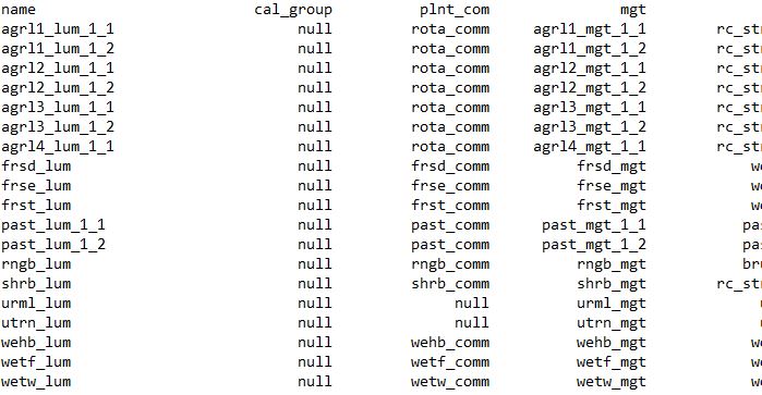
Fig. 9: Screenshot of the rewritten ‘landuse.lum’ file in the SWAT+ project.
The HRUs in the ‘hru-data.hru’ now point to the new land uses in ‘landuse.lum’.
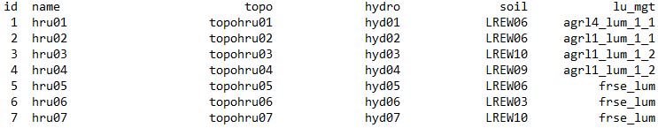
Fig. 10: Screenshot of the rewritten ‘hru-data.hru’ file in the SWAT+ project.
Fig. 11 shows a screenshot of the written operation schedule for
agrl1_mgt_1_1 in ‘schedule.mgt’. You can see that
operations for 6 years (2000 to 2005) were written. The scheduled
operation dates are now selected based on the conditions in the
management input file and the time series of the weather variables and
the additional variable api. I therefore want to stress
that the scheduled operation dates are always linked to the simulation
period, which is controlled by the input file ‘time.sim’. Thus,
‘time.sim’ is always written together with the management
schedule. By manually changing the simulation period in
‘time.sim’ we would loose this link between scheduling
conditions and the time series of the variables.
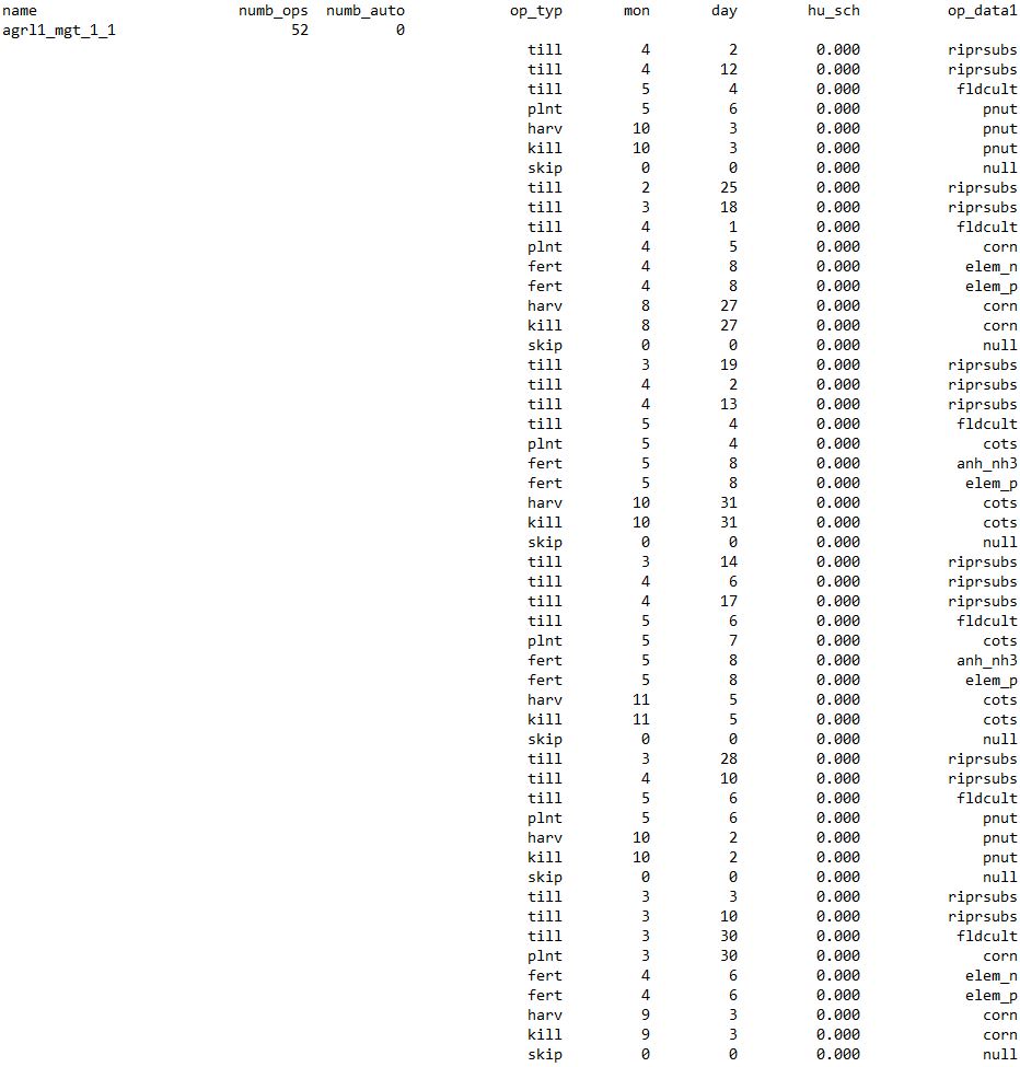
Fig. 11: Screenshot of the rewritten ‘schedule.mgt’ file in the SWAT+ project.
Resetting the SWAT project
Writing the management schedules overwrites the original SWAT project
input files. The farmr project however made a copy of the
initial input files which will be overwritten. With
.$reset_files() you can reset the project to its initial
version.
lrew_demo$reset_files()

#> Resetting all management files:
#>   - Resetting 'hru-data.hru'
#>   - Resetting 'landuse.lum' and 'schedule.mgt'
#>   - Resetting 'time.sim'
#> Finished resetting management files in 0S
This can be for instance relevant if you want to setup a new
farmr project for the initial state of the SWAT model setup
which uses the original land use label without any suffixes. If you
would start a new farmr project with the rewritten
‘landuse.lum’ file, .$read_management() would warn
you that for all land uses that now have a suffix added no managements
are defined in the management input file. To correctly link the land
uses of the HRUs with the operation schedules defined in the management
input file you would have to reset the input files in the SWAT project
folder first.